Bringing the Predator-Prey Model to Life: An Animated Tale
How to animate a simulation in not very many lines of Python code...

I design, build and test things virtually before decisions are made in the real world.
In our previous escapade through the mathematical savannahs, we embarked on a journey to construct the venerable predator-prey model. This time, we're not just charting the numbers; we're breathing life into our simulation. Yes, you read that right. We're animating our predators and prey, turning static graphs into a riveting wildlife documentary, minus David Attenborough's soothing narration.
The Importance of Animation in Simulations
Why animate, you ask? Well, imagine reading about a thrilling football match versus watching the highlights. Animation transforms our understanding from abstract numbers to vivid, intuitive stories. It's the difference between reading the menu and tasting the dish.
This approach is not just about engagement; it's about clarity and insight. For sectors ranging from heavy industry to healthcare, where dynamic systems and complex interactions are the norm, animation can illuminate trends, reveal hidden patterns, and engage stakeholders in a way static data simply cannot. It's a tool for decision-makers to visualise scenarios and make informed choices, bridging the gap between theoretical models and real-world applications.
From Static to Cinematic: The Predator-Prey Model Reimagined
Our previous article laid the groundwork, detailing the nuts and bolts of simulating the delicate dance between rabbits and wolves. Now, we're adding the magic of motion pictures to this ecological epic. Let's dive into the key changes that will transform our static model into a blockbuster animation.
The Revamped display_grid Function
Gone are the days of dual plots that made our simulation look like a split-screen video game. We've merged the rabbit and wolf populations into a single, dynamic heatmap. This isn't just a visual upgrade; it's a narrative choice, highlighting the dramatic interplay between predator and prey on a shared stage.
def display_grid(grid, camera):
# Create a combined grid representation
combined_grid = np.zeros((grid_size, grid_size))
for i in range(grid_size):
for j in range(grid_size):
if grid[i, j].rabbit and grid[i, j].wolf:
combined_grid[i, j] = 3 # Both rabbit and wolf
elif grid[i, j].wolf:
combined_grid[i, j] = 2 # Only wolf
elif grid[i, j].rabbit:
combined_grid[i, j] = 1 # Only rabbit
# Else, it remains 0 (empty)
# Use a colormap that clearly distinguishes between the states, adjust as needed
#cmap = sns.color_palette("light:b", as_cmap=True)
sns.heatmap(combined_grid, ax=ax, cbar=False, cmap=cmap, norm=norm)
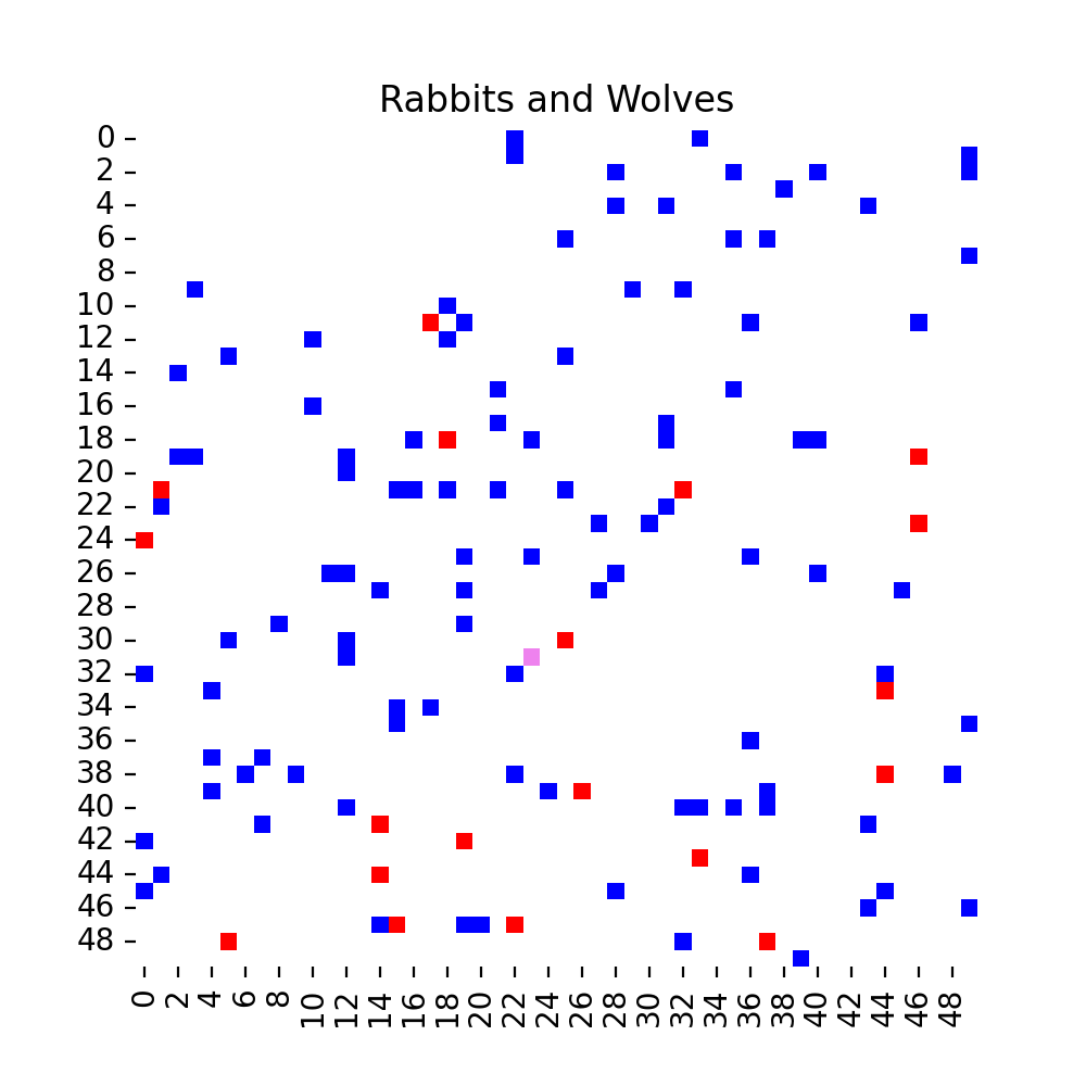
ax.set_title('Rabbits and Wolves')
# Ensure the figure is fully rendered
fig.canvas.draw()
# Take a snapshot after plotting
camera.snap()
A Splash of Colour
To enhance our visual storytelling, we've introduced a custom colour scheme. Rabbits are now represented in a calm blue, wolves in a menacing red, and areas of overlap in a dramatic violet, representing, well, violence. This isn't just for aesthetics; it's a crucial narrative device, instantly conveying the state of the ecological battlefield.
from matplotlib.colors import ListedColormap, BoundaryNorm

# Define your custom colors
colors = ['white', 'blue', 'red', 'violet']  # Corresponding to 0 (empty), 1 (rabbit), 2 (wolf), 3 (both)
cmap = ListedColormap(colors)

# Define the boundaries for your colors
bounds = [0, 1, 2, 3, 4]  # The values used in combined_grid
norm = BoundaryNorm(bounds, cmap.N)
The Magic of Celluloid
And now, the moment we've all been waiting for: bringing our ecological epic to the silver screen of our Python IDEs. With the stage set and our actors (rabbits and wolves, in case you've forgotten) ready for their close-ups, we turn to the magic of Celluloid. This isn't Hollywood's celluloid, mind you, but a Python library that's equally capable of producing blockbusters, at least in the world of agent-based simulations.
from celluloid import Camera

# Initialize the plot and camera
fig, ax = plt.subplots(1, 1, figsize=(5, 5))

camera = Camera(fig)

# Running the simulation and capturing each step
for step in range(simulation_steps):
    grid = simulate_step(grid)
    remove_dead_wolves_fixed(grid)
    display_grid(grid, camera)  # Pass the camera to capture the state

    rabbit_count = sum(grid[i, j].rabbit for i in range(grid_size) for j in range(grid_size))
    wolf_count = sum(grid[i, j].wolf for i in range(grid_size) for j in range(grid_size))

    rabbit_counts.append(rabbit_count)
    wolf_counts.append(wolf_count)

# Creating the animation
animation = camera.animate()

animation.save('predator_prey_simulation.gif', writer='imagemagick')
Our final result simulated for 100 steps...
One Final Note
Animating the predator-prey model isn't just about making pretty pictures. It's about understanding. It's about seeing the invisible dance unfold before our eyes, communicating patterns and behaviours that static graphs struggle to capture. Applied in industry, it's a way to make simulations compelling, to bring otherwise disinterested parties into the fold, and to drive home messaging.


